In this machine problem, you will use simple Bayes (aka naïve Bayes) to learn a distribution for a real-world problem. You will first implement the learning algorithm for simple Bayes, then conduct an experiment with natural language data, and finally, study its potential as a classifier and as a tool for probability estimation.

You will use the naïve Bayes algorithm to solve a classification problem, then conduct your experiments compare two different techniques of probability estimation. One is based on the naïve Bayes assumption, and the second will be estimated directly from the data (or the probability distribution definition).

This data set is provided courtesy of Professor Dan Roth at the University of Illinois at Urbana-Champaign. You will download the training and test examples from the class home page.

This is a collection of examples generated from sentences containing either the word "except" or "accept" in the Wall Street Journal (WSJ). You can see the raw sentences and the examples generated from them on the course web site (in the Homework 2 archive). The sentences were transformed to attribute vector representations (the attributes are small conjunctions of the words and the part of speech information). Aggressive statistical pruning of attributes (preliminary attribute subset selection, or relevance determination) was done to yield only 78 attributes. In each example, we list only the indices of the active attributes.

For this data set, we will investigate 2 different results and the correlation between them.

1. Prediction of naïve Bayes. In order to complete this section you must learn x₁ as a function of the other attributes. After the learning phase (using the 1000 training examples), you need to find the performance of your naïve Bayes classifier on the test data. Train your classifier on the training set, and apply it to the test set to determine the number (and percentage) of examples it predicts correctly.
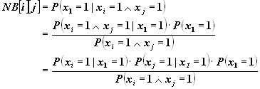
2. Accuracy of density estimation. Here, we compare 2 ways of estimating the empirical density function. You will estimate the conditional probability of the label x₁ given values of any two other attributes. That is, you will find the probability that any example is positive (labeled +) as a function of only 2 attributes at a time. This will be done in two ways: one that uses the naïve Bayes assumption, and one that does not. The density estimation will be done using only the training data.

1. " x_i x_j Î S, estimate the true empirical probability:

P[i][j] = P(x₁ = 1 | x_i = 1 Ù x_j = 1)

2. Next, estimate the empirical probability, assuming the naïve Bayes condition. That is, evaluate:



3. This gives you two probability distributions. You can then compute the distance between them:

1. There are 4 measurements to submit:

1. The accuracy of the naïve Bayes predictor for the data set (training, test) - report both the number of correct predictions and the percentage.
2. For each data set, report the value you get for D(P,B).

1. A brief (2 paragraph) discussion of the results.
2. Your source code.